Many Factors Affecting Optimization
机器学习的一般步骤
Model Bias
- The model is too simple.
- find a needle in a haystack (大海捞针)
- but there is no needle
- Solution: redesign your model to make it more flexible
- more features
- more neurons, layers
Optimization Issue
- Large loss not always imply model bias. There is another possibility …
- A needle is in a haystack…, Just cannot find it.
Model Bias v.s. Optimization Issue
- Gaining the insights from comparison
- 当在测试数据上和训练数据上有着类似的loss曲线时,这说明是
Optimization Issue的问题
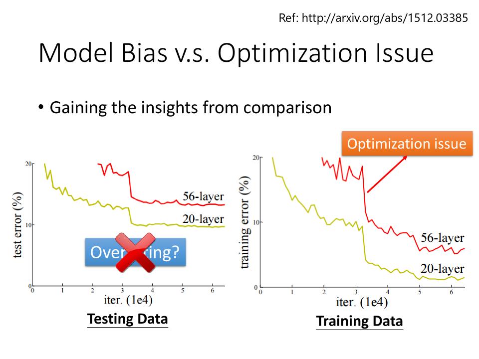
Optimization Issue
- Start from shallower networks(or other models), which are easier to optimize.
- 从更容易优化的较浅的网络(或其他模型)开始。
- If deeper networks do not obtain smaller loss on
training data, then there is optimization issue. - 如果更深的网络在“训练数据”上没有获得更小的损失,那么就存在优化问题。
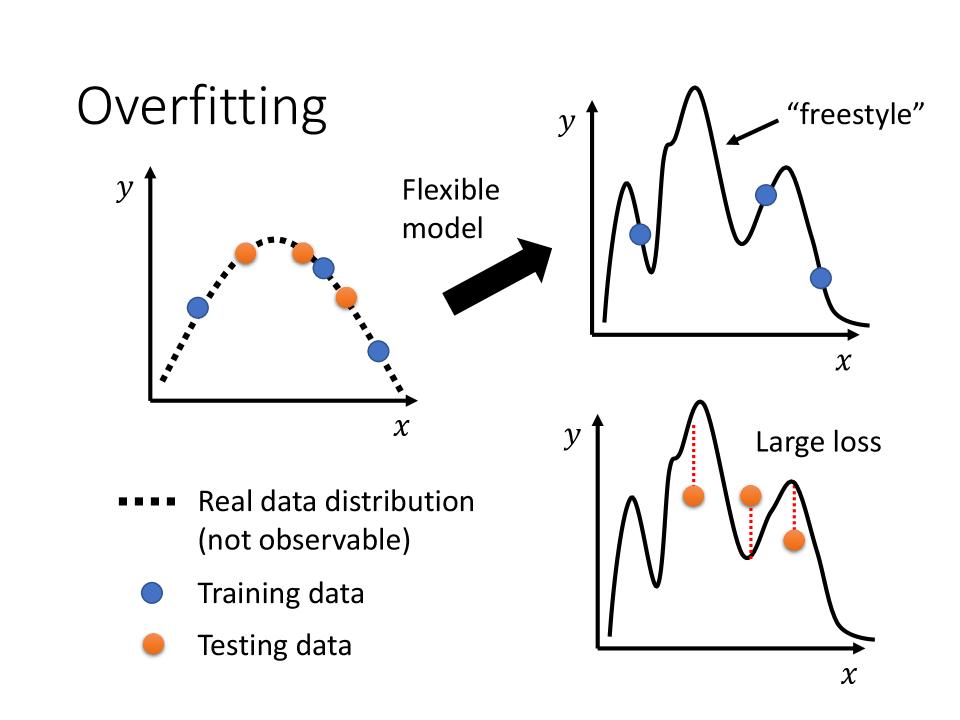
Overfitting
- Small loss on training data, large loss on testing data. Why?
- 数据分布的这条虚线通常是无法明确的获知的,我们通常只能拿到在这条曲线上的多个
Training Data - 由于model的Flexible, 训练出来的这个模型,在没有训练数据的地方会有“freestyle”, 从而导致测试数据的overfitting
- 增加训练数据
- Data augmentation(用一些对这个问题的理解,自己创造出新的训练数据。例如:对图片左右反转,或者是截取其中一块等)
- 通过限制model来解决overfitting,给model制造限制的方法:
- make your model simpler
- Less parameters, sharing parameters
- Fully-connected的架构是一个比较有弹性的架构;而CNN是一个比较有限制的架构(根据影像的特性来限制模型的弹性)
- Less features
- Early stopping
- Regularization
- Dropout
- 这里需要注意,太多的限制和太简单的模型会导致
model bias
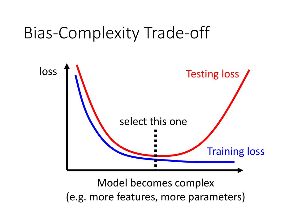
Bias-Complexity Trade-off
- 通过观察
Training loss和Testing loss的loss曲线来选择model和对应的模型限制
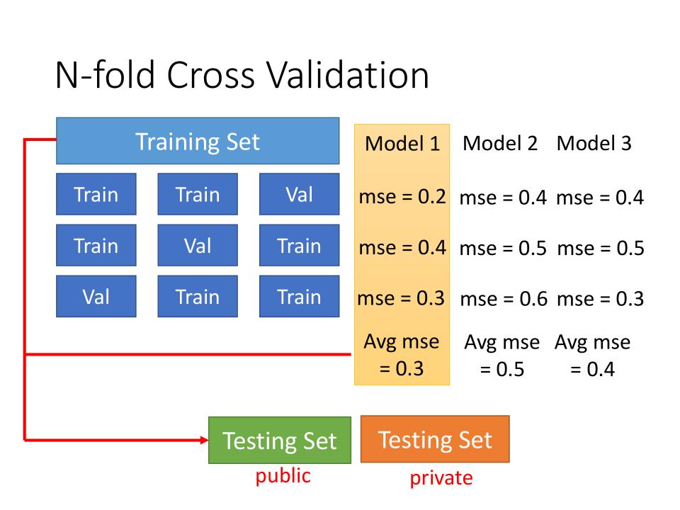
N-fold Cross Validation
- Cross Validation就是N-flod Cross Validation的一个特例
- 如果使用
Cross Validation, 则使用Validation Set的loss最小进行模型的选择 - 当使用
N-fold Cross Validation时,则使用mse的avg最小来挑选模型
Mismatch
- Your training and testing data have different distributions.
- 需要对训练资料和测试资料有一定的了解才能分清到底是不是mismatch
- mismatch和overfitting不是一个东西,overfitting可以通过增加训练资料来解决,而mismatch无法通过增加训练资料来解决
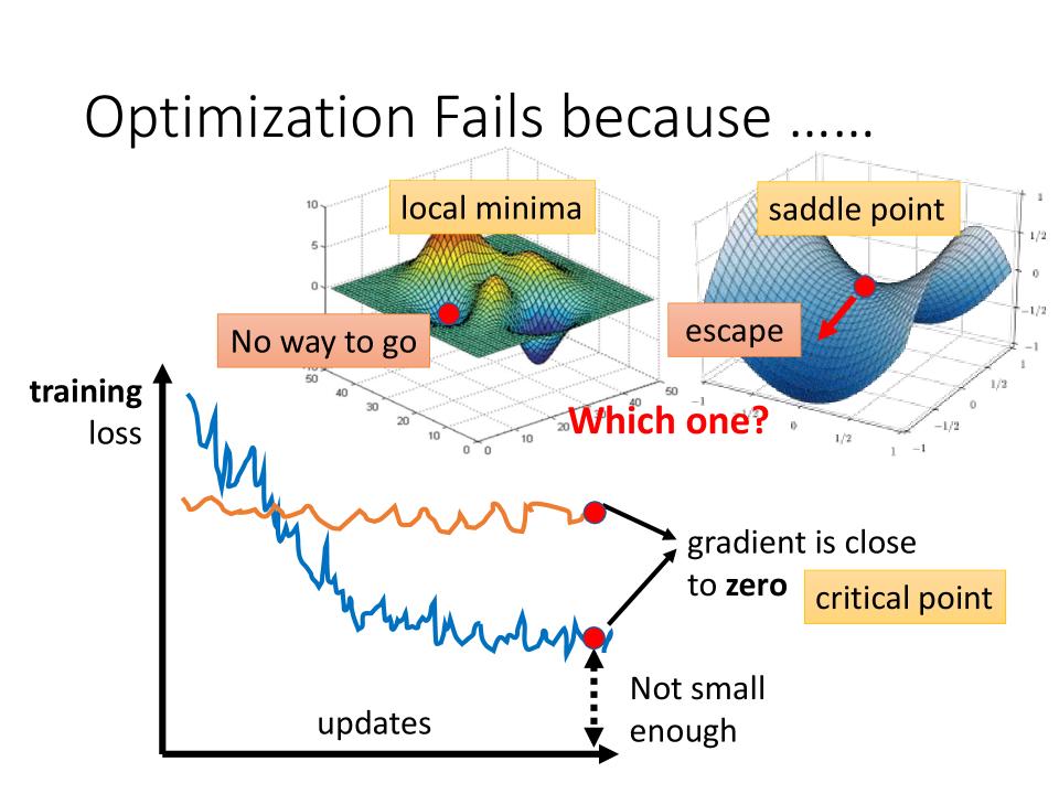
Optimization Fails because
- loss is
Not small enough, because the gradient is close to zero. - Gradient为零的情况有:
local minima,local maxima,saddle point等 saddle point: Gradient为零, 同时既不是local minima也不是local maxima的地方- Gradient为零的点统称为
critical point
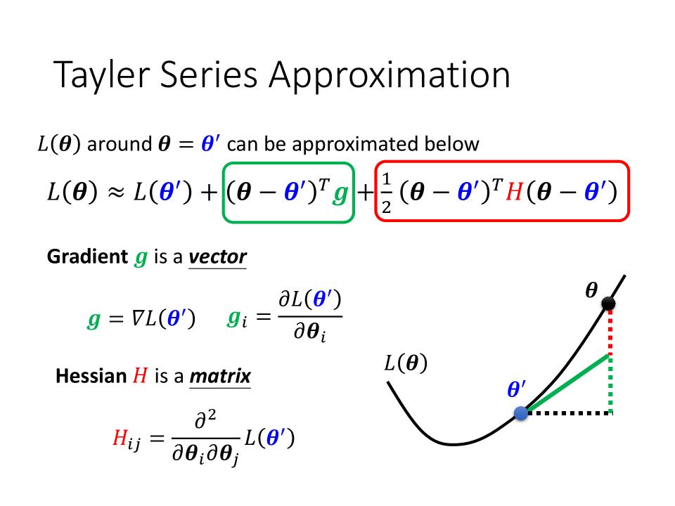
Tayler Series Approximation(泰勒级数逼近)
- 如何知道一个
critical point是local minima还是saddle point - 其中包括 Gradient $\color{green}g$ is a vector, Hessian $\color{red}H$ is a matrix.
Hessian
- Gradient $\color{green}g$ 为0时,则可知目前所在位置为临界点
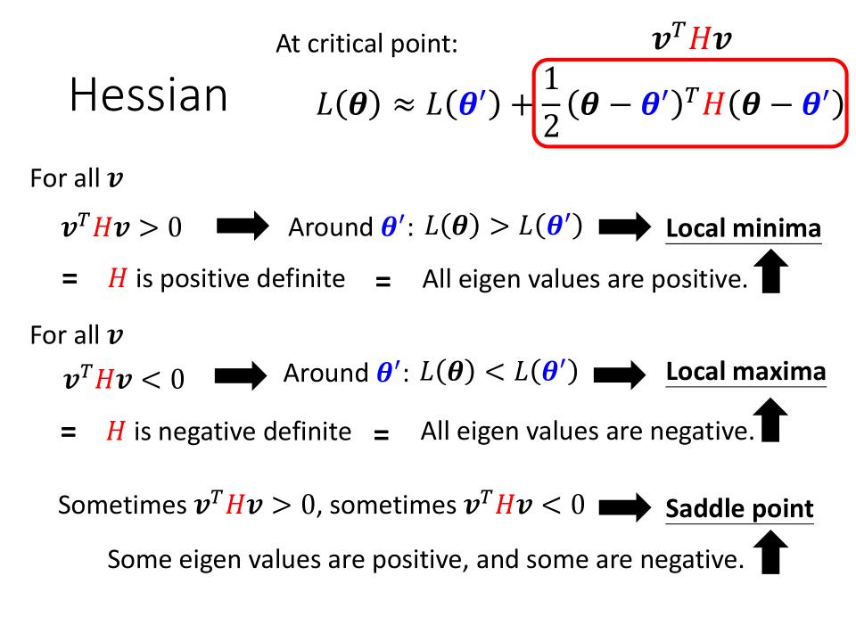
Critical Point - Hessian $\color{red}H$ can telling the properties of critical points.
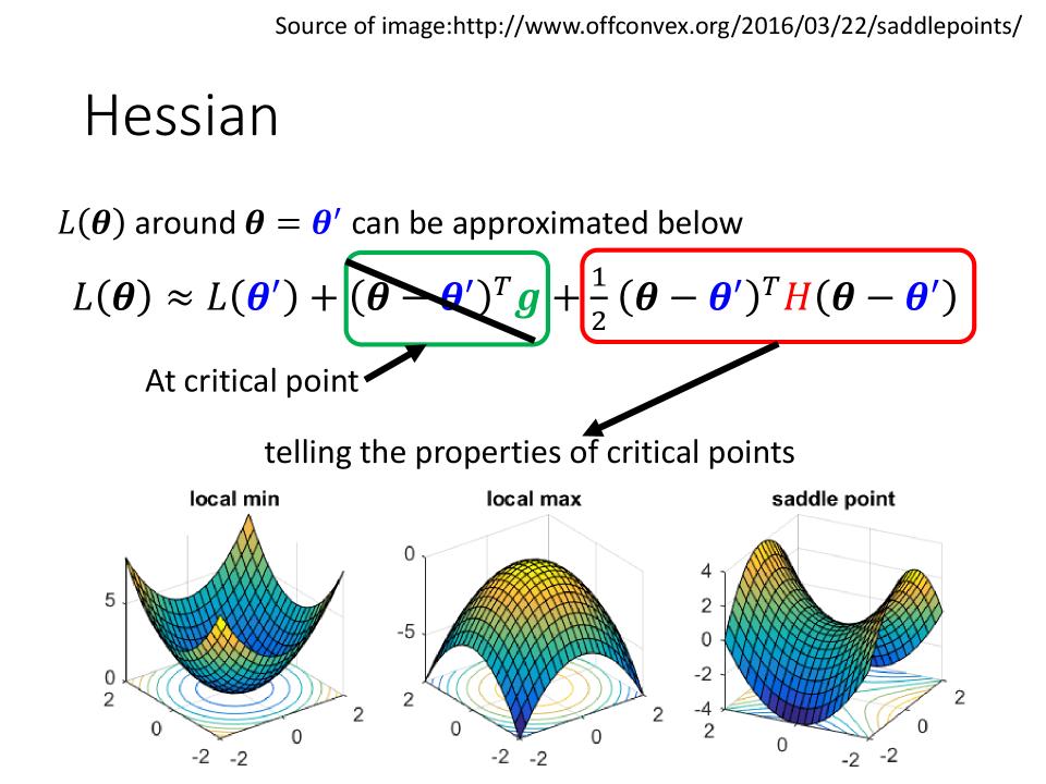
- 当$\color{red}H$这个矩阵中的值全部为正值,则当前所在为
Local Minima - 当$\color{red}H$这个矩阵中的值全部为负值,则当前所在为
Local Maxima - 当$\color{red}H$这个矩阵中的值有正有负,则当前所在为
Saddle Point
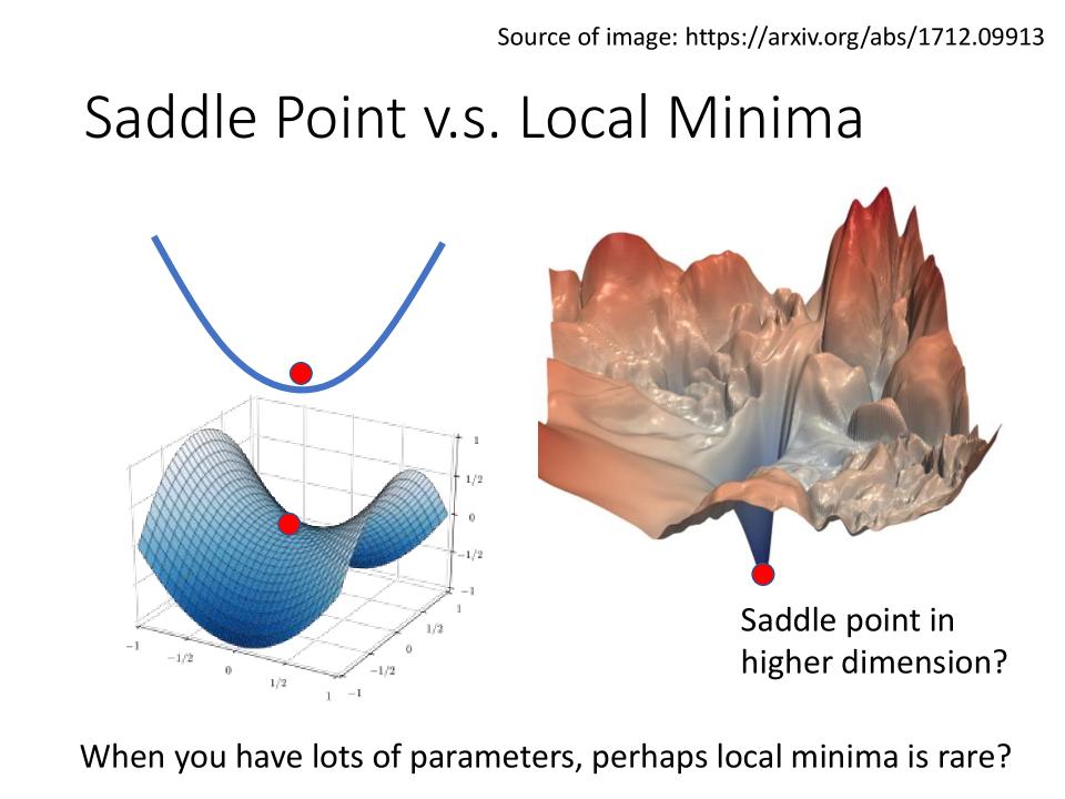
Saddle Point v.s. Local Minima
- 在一维的空间中看到的local minima,在二维的空间中看到的可能就只是saddle point.
- 当我们有更多的参数,也许local minima是很少见的
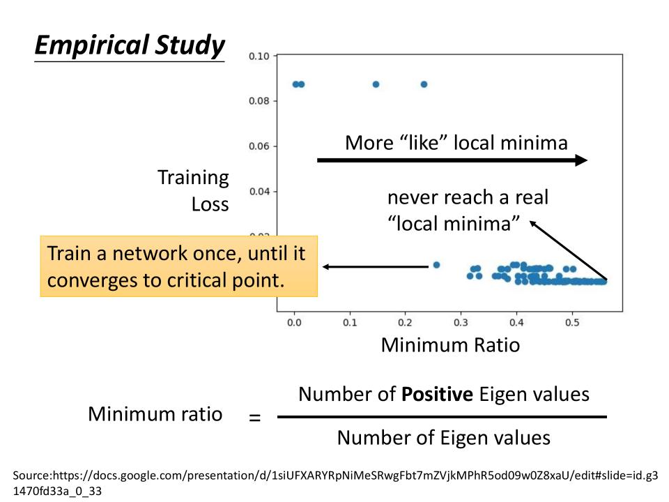
Minimum Ratio
- 是所有
Local Minima的数量与所有Critical Point的比值 - 从图上可知,最大的ratio也只是0.6
- 图上Eigen Values就是前文所说的Hessian Matrix.
Batch
- 不会拿所有的资料去算微分,会把所有的资料分成很多个batch,
- 每个batch的资料算一个loss,算一个Gradient再update参数
- 所有的资料算过一遍叫做一个epoch
shaffleafter each epoch,shaffle有很多不同的做法:- 一个常见的做法是在每个epoch开始之前,会分一次batch,每一个epoch的batch都不一样
Small Batch v.s. Large Batch
- Consider we have 20 examples(N=20)
- Batch size = N (Full batch)
- Update after seeing all the 20 examples
- Long time for cooldown but powerful
- Batch size = 1
- Update for each example, Update 20 times in an epoch
- Short time for cooldown but noisy
由于有GPU的平行运算的能力,从性能的角度出发得到如下结论:
- Larger batch size does not require longer time to compute gradient(unless batch size is too large)
- Smaller batch requires longer time for one epoch (longer time for seeing all data once)
从准确率来看
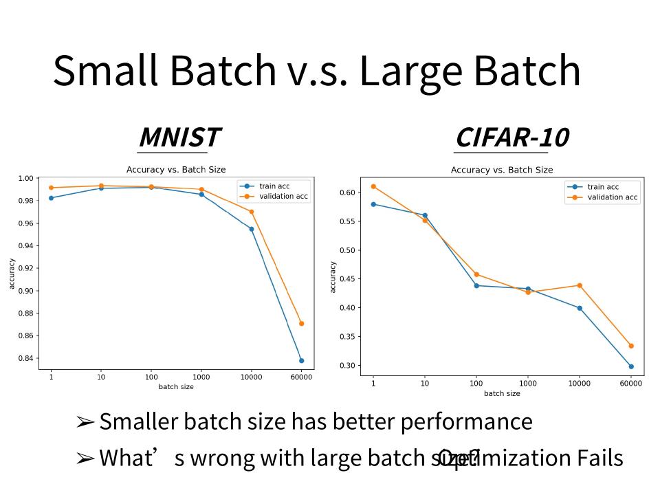
- 反而是有noisy的batch可以得到好的结果。Smaller batch size has better performance.
- 如下图,横轴是batch size,纵轴是正确率。如图可知batch size越大,validation set上的结果越差。
- 这个是overfitting么?这个不是overfitting, 因为我们用的数据和模型都是一致的。所以这里发生在larger batch size上的情况是Optimization Fails.
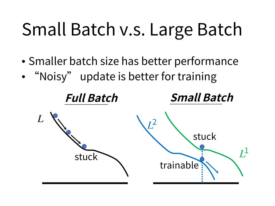
为什么在Noisy的batch size上update更好呢?一种可能的解释是:
- Full Batch比较容易stuck,而Small Batch由于不同batch的数据有所不同,所以相对来说不太容易stuck,更容易train到比较小的loss
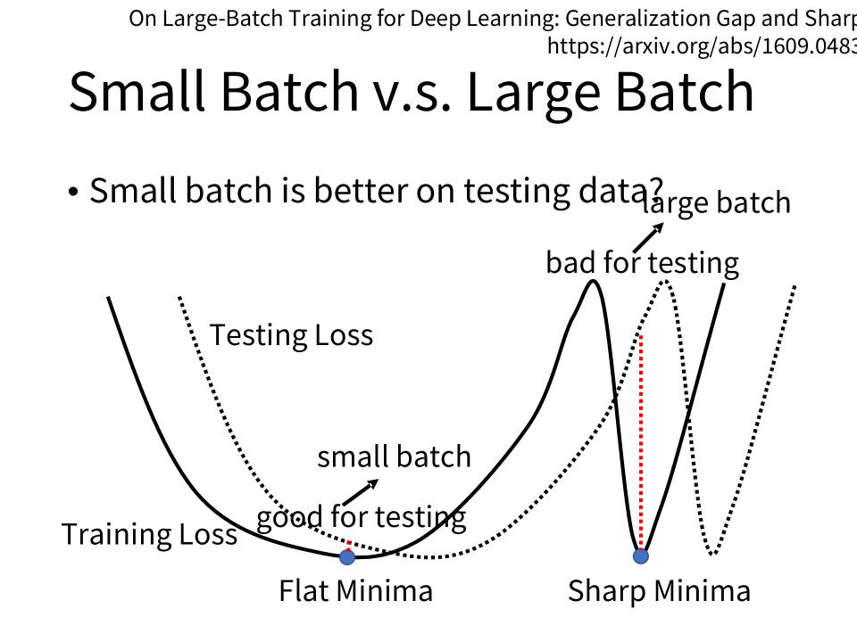
有研究表明,小的batch size不仅针对training有效,在testing的时候也比大的batch size要好。如下图:
- 数据相同,模型相同的情况下,将大的batch size在training set上的accuracy调整的和小的batch size一样
- 而从图上右侧表格观察,LB的accuracy比SB的accuracy要差,这是overfitting
- 详见资料: On Large-Batch Training for deep Learning: Generalization Gap and Sharp Minima

为什么会有这种现象呢?
- 假设如下图的training loss上有很多个Local Minima,这些Local Minima的Loss都足够小
- 但是Local Minima还是有好坏之分的。如图中,Flat minima(盆地)的容错性要优于sharp minima(峡谷)。
- 大的batch size倾向于走到峡谷里面,而小的batch size倾向于走到盆地里面。
- 小的batch size有很多的noisy,它每次走的方向都不太一样,如果这个峡谷比较的窄,那么noisy的batch size很容易跳出峡谷。
| Small | Large | |
|---|---|---|
| Speed for one update (no parallel) | Faster | Slower |
| speed for one update (with parallel) | Same | Same(not too large) |
| Time for one epoch | Slower | Faster |
| Gradient | Noisy | Stable |
| Optimization | Better | Worse |
| Generalization | Better | Worse |
兼顾速度与Generalization的研究文章
- Large Batch Optimization for Deep Learning: Training BERT in 76 minutes
- Extremely Large Minibatch SGD: Training ResNet-50 on ImageNet in 15 Minutes
- Stochastic Weight Averaging in Parallel: Large-Batch Training that Generalizes Well
- Large Batch Training of Convolutional Networks
- Accurate, Large Minibatch SGD: Training ImageNet in 1 Hour
Momentum
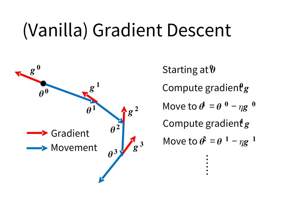
(Vanilla) Gradient Descent
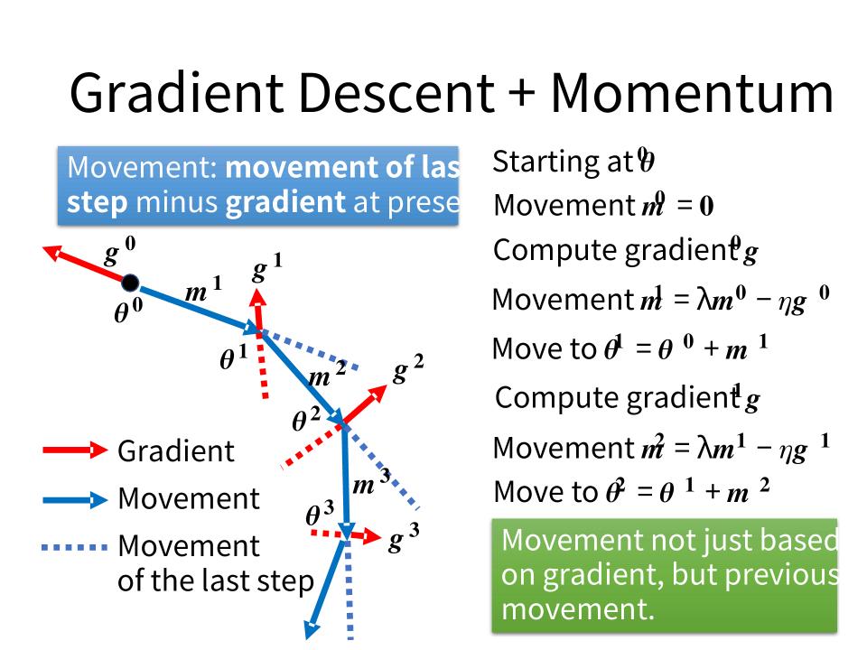
Gradient Descent + Momentum
- Movement: movement of last step minus gradient at present
Adaptive Learning Rate
- $ \text{Training stuck} \ne \text{Small Gradient} $
- 当loss不再下降的时候,需要确认一下Gradient是否为0;即loss不再下降需要分析stuck的原因
- 如图,当loss不再下降时,norm of gradient 并没有为0
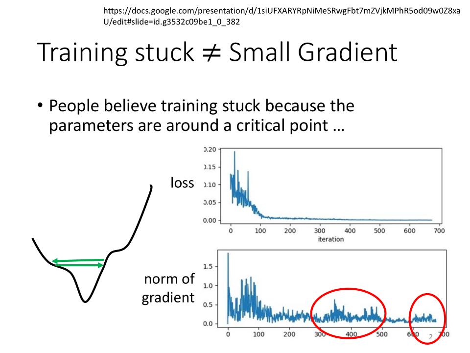
Training can be difficult even without critical points.
- Learning rate cannot be one-size-fits-all(一刀切).
- Different parameters needs different learning rate.
- 相对平坦的Gradient Descent需要较大的Learning Rate
- 相对尖锐的Gradient Descent需要较小的Learning Rate
Formulation for one parameter:
\begin{align} \theta_i^{t+1} & \leftarrow \theta_i^t - {\color{red}\eta}g_i^t \cr g_i^t & = \frac{\partial L}{\partial \theta_i} |_{\theta=\theta^t} \cr & \Downarrow \cr \theta_i^{t+1} & \leftarrow \theta_i^t - {\color{red}\frac{\eta}{\sigma_i^t}}g_i^t \end{align}
${\color{red}\frac{\eta}{\sigma_i^t}}$就是Parameter dependent的Learning Rate,下面介绍几种常见的计算方法:
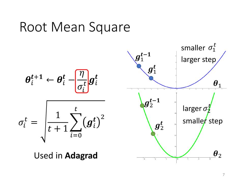
Root Mean Square (Used in Adagrad)
\begin{align} \theta_i^1 & \leftarrow \theta_i^0 - \frac{\eta}{\sigma_i^0}g_i^0 & \sigma_i^0 &= \sqrt{(g_i^0)^2} = |g_i^0| \cr \theta_i^2 & \leftarrow \theta_i^1 - \frac{\eta}{\sigma_i^1}g_i^1 & \sigma_i^1 &= \sqrt{\frac{1}{2}[(g_i^0)^2+(g_i^1)^2]} \cr \theta_i^3 & \leftarrow \theta_i^2 - \frac{\eta}{\sigma_i^2}g_i^2 & \sigma_i^2 &= \sqrt{\frac{1}{3}[(g_i^0)^2+(g_i^1)^2+(g_i^2)^2]} \cr & \vdots \cr \theta_i^{t+1} & \leftarrow \theta_i^t - \frac{\eta}{\sigma_i^t}g_i^t & \sigma_i^t &= \sqrt{\frac{1}{t+1}\sum_{i=0}^t(g_i^t)^2} \end{align}
- 小的$\sigma_i^t$会有大的step
- 大的$\sigma_i^t$会有小的step
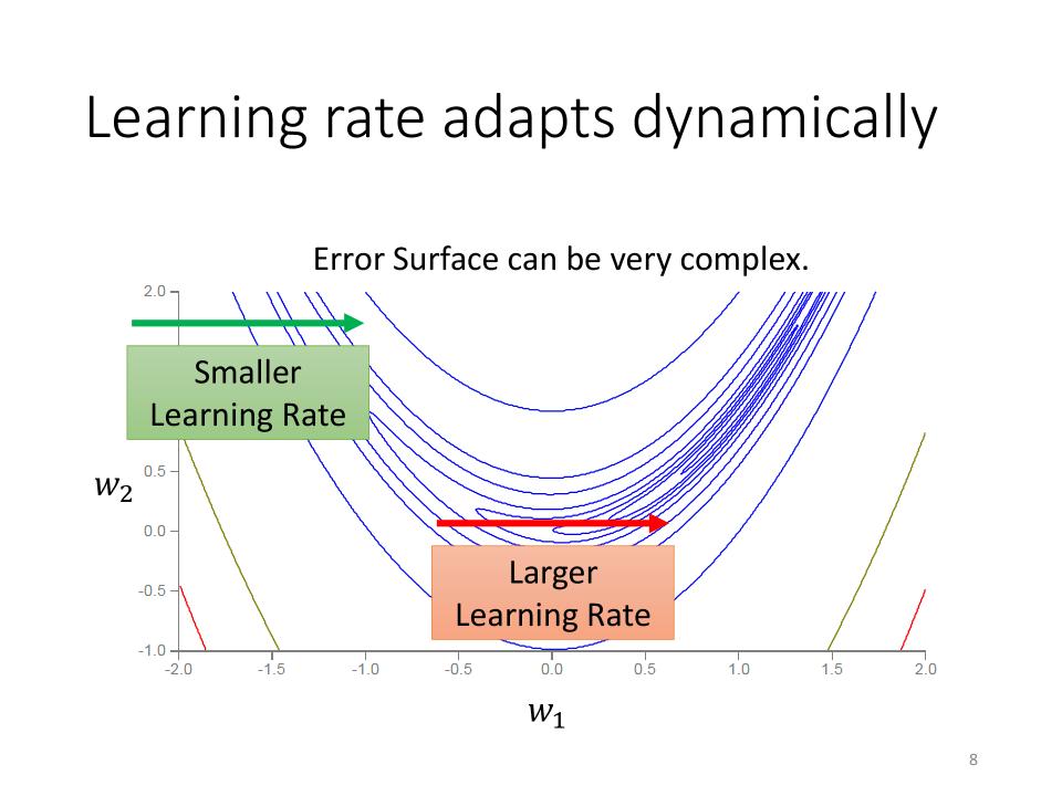
Learning rate adapts dynamically
- 即使针对同一个参数,在不同的时候,可能也需要有不同的Learning Rate
RMSProp
\begin{align} \theta_i^1 & \leftarrow \theta_i^0 - \frac{\eta}{\sigma_i^0}g_i^0 & \sigma_i^0 &= \sqrt{(g_i^0)^2} = |g_i^0| \cr & & & \text{设 } 0 < \alpha < 1 \cr \theta_i^2 & \leftarrow \theta_i^1 - \frac{\eta}{\sigma_i^1}g_i^1 & \sigma_i^1 &= \sqrt{\alpha(\sigma_i^0)^2 + (1-\alpha)(g_i^1)^2} \cr \theta_i^3 & \leftarrow \theta_i^2 - \frac{\eta}{\sigma_i^2}g_i^2 & \sigma_i^2 &= \sqrt{\alpha(\sigma_i^1)^2 + (1-\alpha)(g_i^2)^2]} \cr & \vdots \cr \theta_i^{t+1} & \leftarrow \theta_i^t - \frac{\eta}{\sigma_i^t}g_i^t & \sigma_i^t &= \sqrt{\alpha(\sigma_i^{t-1})^2 + (1-\alpha)(g_i^t)^2} \end{align}

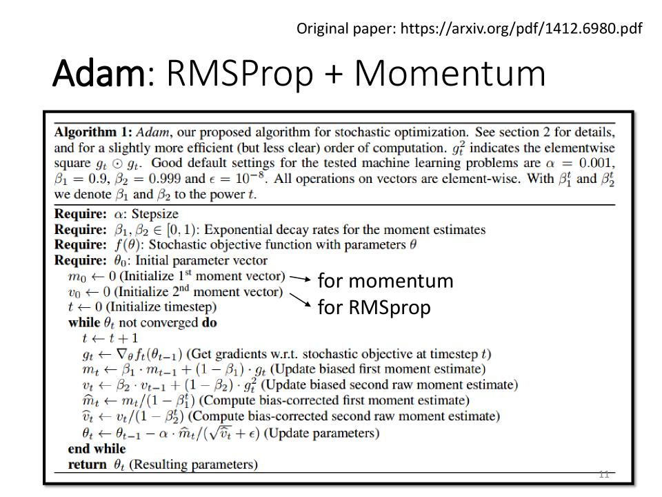
Adam: RMSProp + Momentum
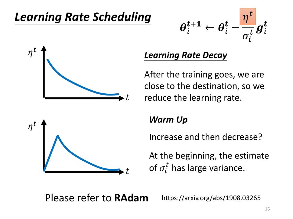
Learning Rate Scheduling
- Learning Rate Decay
- After the training goes, we are closer to the destination, so we reduce the learning rate.
- Warm Up
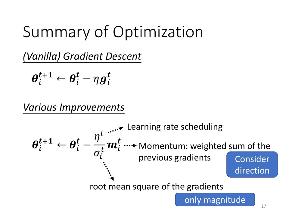
Summary Of Optimization
- Momentum: weighted sum of the previous gradients (考虑方向)
- $\sigma_i^t$: 只考虑大小不考虑方向
- $\eta^t$: Learning rate scheduling
Loss for Classification
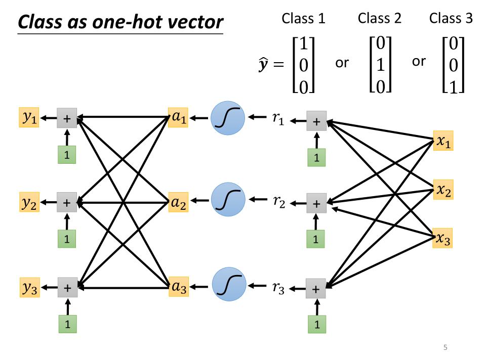
Class as one-hot vector
- one-hot vector for multi-output
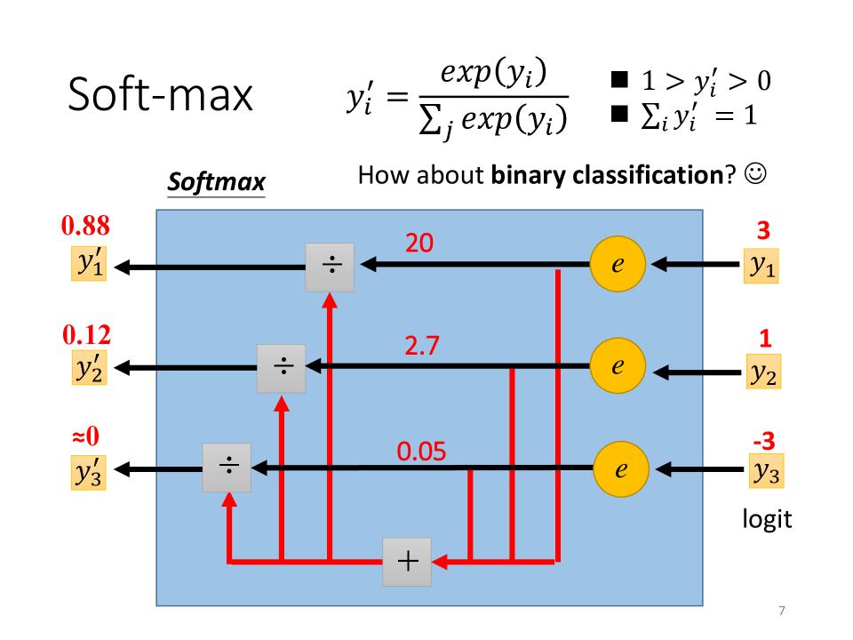
Soft-max
- soft-max对上层多输出结果做一个normalize
- 并且让大的值和小的值之间的差距更大
- soft-max有时又叫做logit
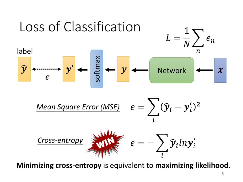
Loss function
- Mean Square Error (MSE): $ e = \sum\limits_i(\hat y_i - y_i^\prime)^2 $
- Cross-entropy: $ e = -\sum\limits_i \hat y_i ln y_i^\prime $
- Minimizing cross-entropy is equivalent to maximizing likelihood.
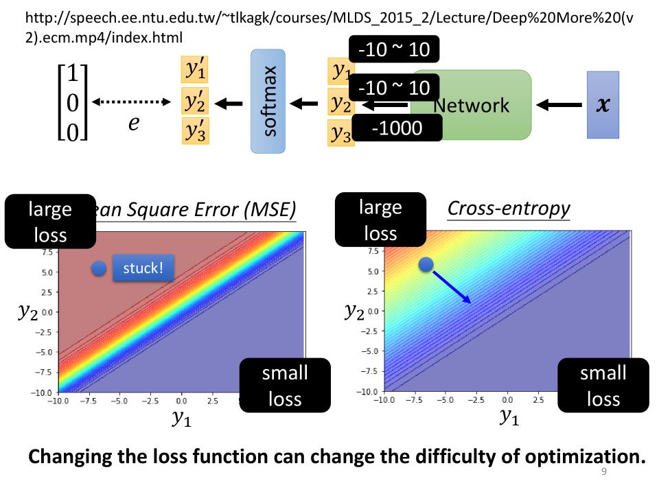
Loss function affect Optimization
- 设目前做一个三分类的模型,当前这个分类的结果是$ \hat y = \begin{bmatrix}1 \cr 0 \cr 0 \end{bmatrix} $
- e表示$y到\hat y$之间的距离,可以是MSE,也可以是Cross-entropy
- $y_1$的取值范围为[-10, 10], $y_2$的取值范围为[-10, 10], $y_3$的取值为固定值-1000
- 下图左右分别为MSE和Cross-entropy想对于y的取值的Error Surface,
- 这两张图中Error Surface的特点都是右下角loss小,左上角loss大
- 假设我们开始的地方都是左上角:如果我们选择Cross-entropy,左上角的地方是有斜率的,所以可以通过gradient的方法一路向右下角走达到small loss; 如果我们选择MSE,我们就卡住了,在MSE左上角这个loss很大的地方,它的gradient非常小,趋进于零,而距离目标又很远,没有很好的办法通过gradient的方法走到右下角。
- 所以如果做classification时,选择使用MSE做loss时,有很大可能性train不起来; 当然如果使用类似Adam这些好的Optimizer时,也许有机会走到右下角。
- Changing the loss function can change the difficulty of optimization.
Normalization
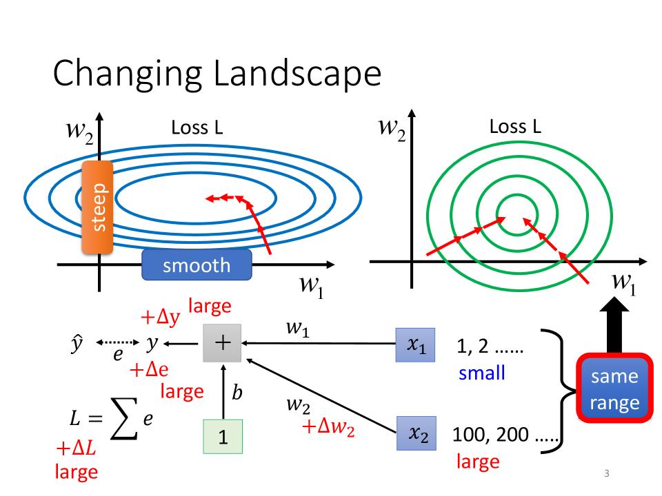
Changing Landscape
- $w_1, w_2$与不同的feature相关,由于不同的feature范围不同,导致了$w_1, w_2$的变动对最终的loss产生不同的影响
- 是否可以找到一个方法,让不同的feature有着相似的range
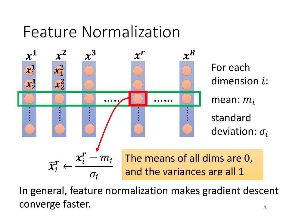
Feature Normalization
- 下图只是Feature Normalization的一种可能
- $ x^1, x^2, \cdots, x^R $ 为数据的R个features
- For each dimension i:
- $m_i$ : mean
- $\sigma_i$ : standard deviation
- Normalization: $\tilde{x}_i^r \leftarrow \frac{x_i^r-m_i}{\sigma_i} $
- The means of all dims are 0, and the variances are all 1
- In general, feature normalization makes gradient descent converge faster.
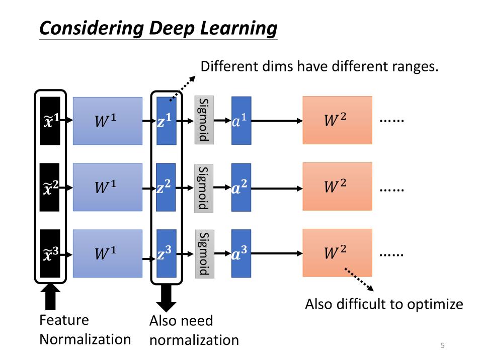
$\theta$的Normalization
- $\tilde{x}^1$在经过$W^1$后得到的$z^1$也是具有不同的range的,这将导致针对$W^2$的optimize会比较的困难
- 对于$W^2$来说,这里的z或者a也是feature,所以这里需要考虑对z或者a做Normalization
- 那么到底在激活函数的前面还是后面做normalization呢?实作中都可以,但当activation function为Sigmoid时,建议在Sigmoid的前面,也就是这里的z做normalization。
Feature Normalization的计算
- $\mu = \frac{1}{n}\sum\limits_{i=1}^nz^i $
- $ \sigma = \sqrt{\frac{1}{n}\sum\limits_{i=1}^n(z^i-\mu)^2} $
- $ \tilde{z}^i = \frac{z^i-\mu}{\sigma} $
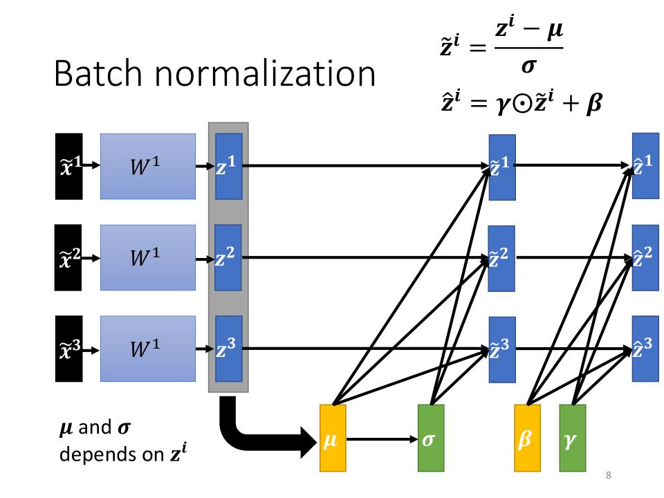
Batch normalization
- 由于需要对$x, z^1, z^2, \cdots, z^n$都做normalization,所以这是一个巨大的network,如果使用这个巨大的network针对所有的数据去求$\mu和\sigma$是不太现实的, 所以只能将范围缩小到一个batch,从而诞生了batch normalization。
- 而在做Batch normalization的时候,往往还会加上一个$\beta和\gamma$, 得到方程$ \hat{z}^i = \gamma\odot\tilde{z}^i+\beta $ 其中 $ \tilde{z}^i = \frac{z^i-\mu}{\sigma} $
- 实际在做训练时,考虑到normalization的情况,在初始情况下$\gamma$会被初始化为one vector(全1的向量), 而$\beta$会被初始化为zero vector(全0的向量)。
Batch normalization - Testing
- We do not always have batch at testing stage.
- Computing the moving average of $\mu$ and $\sigma$ of the batches during training.
- 如下计算出$\bar{\mu}, \bar{\sigma}$,替换training中的表达式$ \tilde{z} = \frac{z-\mu}{\sigma} $得到$ \tilde{z} = \frac{z-\bar{\mu}}{\bar{\sigma}} $
- How to compute moving average?
\begin{align} \mu^1, \mu^2, \mu^3, \cdots, \mu^t \cr \bar{\mu} \leftarrow p\bar{\mu} + (1-p)\mu^t \end{align}
Batch Normalization Refs
- Batch Normalization: Accelerating Deep Network Training by Reducing Internal Covariate Shift
- How Does Batch Normalization Help Optimization
- Experimental results (and theoretically analysis) support batch normalization change the landscape of error surface.
- This suggests that the positive impact of BatchNorm on training might be somewhat serendipitous(偶然的,发现了一个意料之外的东西).
Normalization Refs
- Batch Renormalization: Towards Reducing Minibatch Dependence in Batch-Normalized Models
- Layer Normalization
- Instance Normalization: The Missing Ingredient for Fast Stylization
- Group Normalization
- Weight Normalization: A Simple Reparameterization to Accelerate Training of Deep Neural Networks
- Spectral Norm Regularization for Improving the Generalizability of Deep Learning
New Optimization
What you have known before?
- SGD - stochastic gradient descent: 随机梯度下降
- SGDM - stochastic gradient descent with momentum
- Adagrad
- RMSProp
- Adam
Some Notations
- $\theta_t$: model parameters at time step t
- $\nabla L(\theta_t) \text{or } g_t$: gradient at $\theta_t$, used to compute $\theta_{t+1}$
- $m_{t+1}$: momentum accumulated from time step 0 to time step t, which is used to compute $\theta_{t+1}$
\begin{align} g_t \cr \overleftarrow{x_t \rightarrow \theta_t \rightarrow y_t ^\underleftrightarrow{L(\theta_t;x_t)} \hat{y}_t} \end{align}
What is Optimization about ?
- Find a $\theta$ to get the lowest $\sum_x L(\theta; x)$ !!
- Or, Find a $\theta$ to get the lowest $L(\theta)$ !!
On-line vs Off-line learning
- On-line: one pair of $(x_t, \hat{y}_t)$ at a time step
- Off-line: pour all $(x_t, \hat{y}_t)$ into the model at every time step
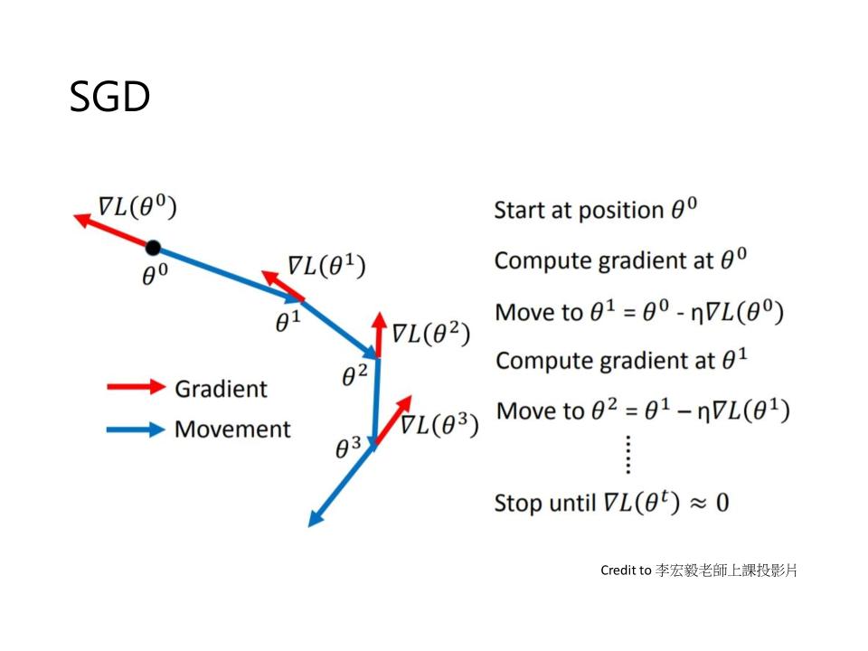
SGD (stochastic gradient descent)
- Start at position $\theta^0$
- Compute gradient at $\theta^0$
- Move to $\theta^1 = \theta^0 - \eta \nabla L(\theta^0)$
- Compute gradient at $\theta^1$
- Move to $\theta^2 = \theta^1 - \eta \nabla L(\theta^1)$
- Stop until $\nabla L(\theta^t) \approx 0$
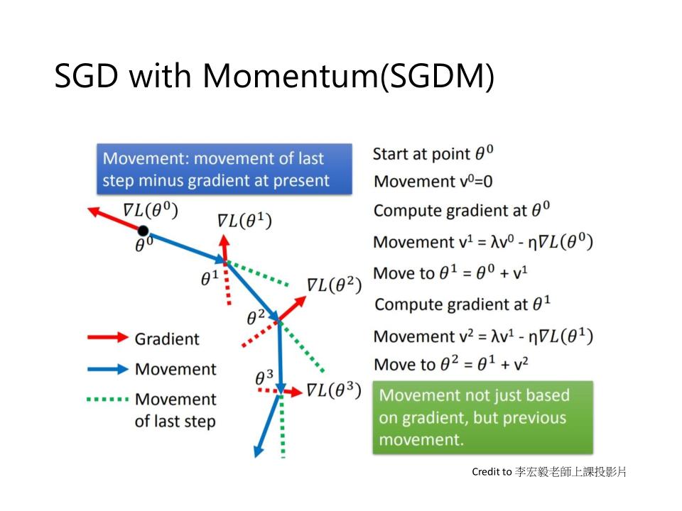
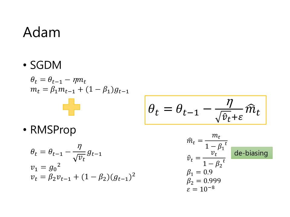
SGDM (stochastic gradient descent with momentum)
- Start at point $\theta^0$
- Movement $V^0=0$
- Compute gradient at $\theta^0$
- Movement $V^1=\lambda V^0 - \eta \nabla L(\theta^0)$
- Move to $\theta^1 = \theta^0 + V^1$
- Compute gradient at $\theta^1$
- Movement $V^2 = \lambda V^1 - \eta \nabla L(\theta^1)$
- Move to $\theta^2 = \theta^1 + V^2$
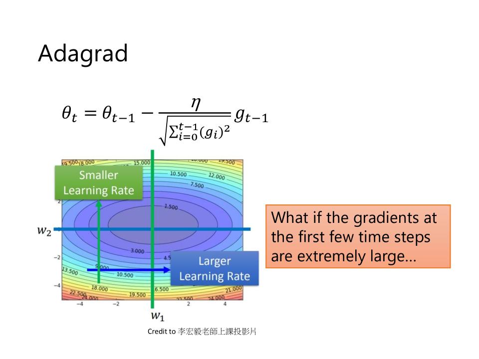
Adagrad
- $\theta_t = \theta_{t-1} - \frac{\eta}{\sqrt{\sum_{i=0}^{t-1}(g_i)^2}}g_{t-1}$
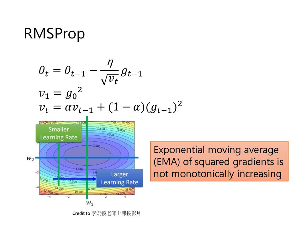
RMSProp
- $\theta_t = \theta_{t-1} - \frac{\eta}{\sqrt{v_t}}g_{t-1}$
- $v_1 = g_0^2$
- $v_t = \alpha v_{t-1} + (1-\alpha)(g_{t-1})^2$
Adam
- $ \theta_t = \theta_{t-1} - \frac{\eta}{\sqrt{\hat{v}_t} + \varepsilon}\hat{m}_t $
Optimizers: Real Application
- BERT: 作Q/A, 文章生成, 2018年提出,使用 ADAM
- Transformer: 用于翻译, 使用 ADAM
- Tacotron: 最早使用神经网络作逼真的语音生成的模型, 2017年提出, 使用 ADAM
- Yolo: 使用 SGDM
- Mask R-CNN: 使用 SGDM
- ResNet: 使用 SGDM
- Gig-GAN: 生成影像, 使用 ADAM
- MEMO: 在不同的分类任务中学到共同的资讯, 使用 ADAM
Adam vs SGDM
- Adam: fast training, large generalization gap, unstable
- SGDM: stable, little generalization gap, better convergence(?)
Simply combine Adam with SGDM?
- SWATS: Begin with Adam(fast), end with SGDM
Towards improving Adam
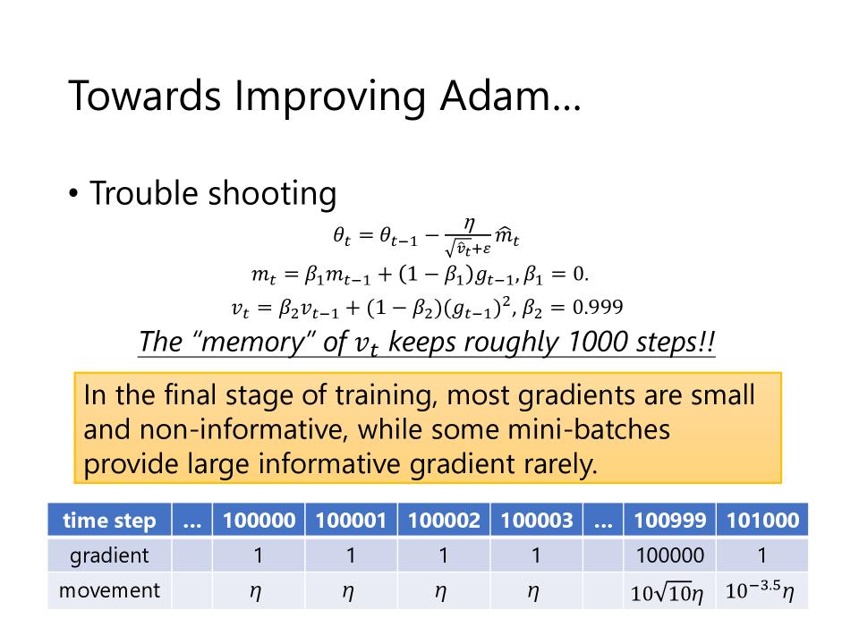
Troubleshooting
- 根据前面的计算公式,从100000到100998的梯度都是1,所以movement都是$\eta$
- 第100999步的梯度很大,100000,对应的movement为$10\sqrt{10}\eta$
- 这导致了前面很多无用的批次的梯度产生了约1000$\eta$的无用变化(乱走),而其中一个有用的很小的批次带来的变化只有33个$\eta$
- 当梯度大部分都很小时,就会产生这样的问题;有用的大的梯度对应的批次会被大量的小的无用的梯度牵着鼻子走
AMSGrad
- Reduce the influence of non-informative gradients
- Remove de-biasing due to the max operation
- 这个算法的改进可以类比为Adagrad和RMSProp, 所以感觉并没有起到很好的效果
Troubleshooting
- In the final stage of training, most gradients are small and non-informative, while some mini-batches provide large informative gradient rarely
- Learning rates are either extremely large(for small gradients) or extremely small(for large gradients)
AdaBound
- AMSGrad only handles large learning rates
- AdaBound的公式中,有参数并非adaptive的,而是有点工程方法
Towards Improving SGDM
- Adaptive learning rate algorithms: dynamically adjust learning rate over time
- SGD-type algorithms: fix learning rate for all updates… too slow for small learning rates and bad result for large learning rates
- There might be a “best” learning rate?
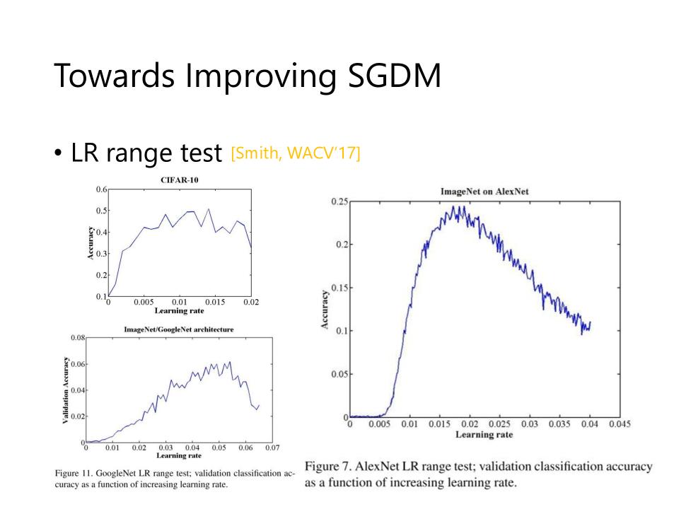
Learning Rate range test
- Learning Rate 在很大或很小的时候,性能都不会很好
- Learning Rate 适中的时候,性能才比较好
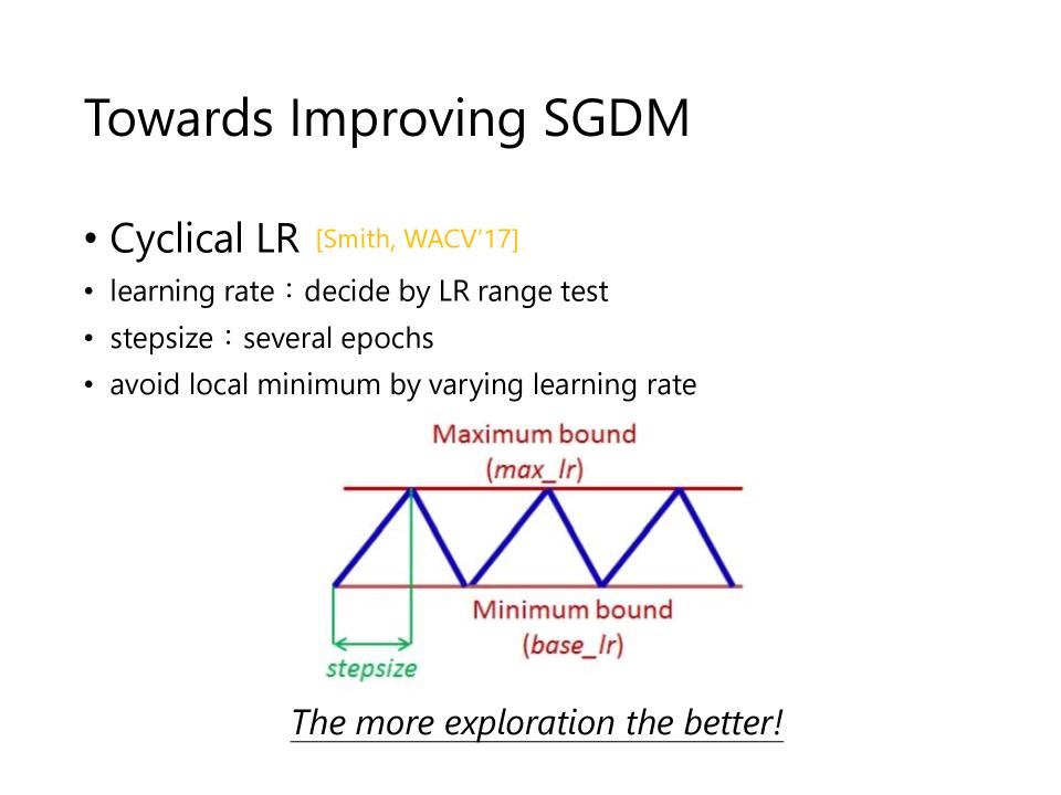
Cyclical LR
- learning rate: decide by LR range test
- step size: several epochs
- avoid local minimum by varying learning rate
- learning rate在大小,大小的循环进行变化
- 变大的时候时在作exploration(探索),变小的时候是在作收敛
- The more exploration the better!
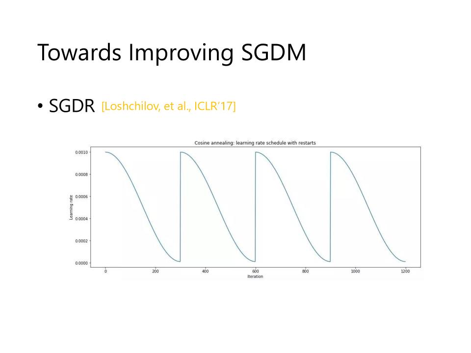
SGDR
- 不用象Cyclical LR一样不断的变大再变小,而是在变小后,重新变回初始值重新开始
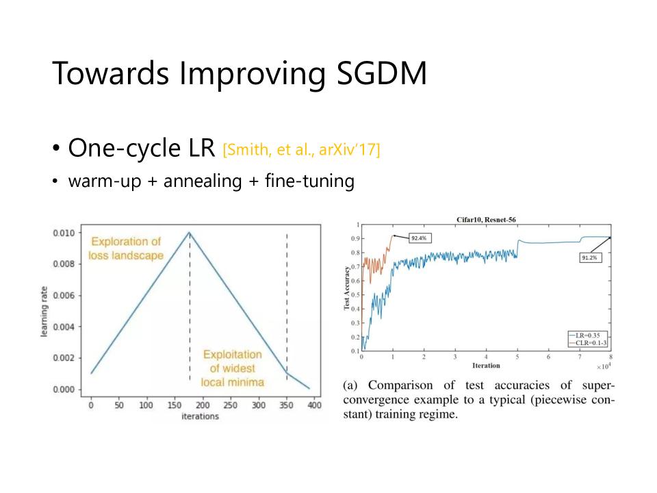
One-Cycle LR
- warm-up + annealing + fine-tuning
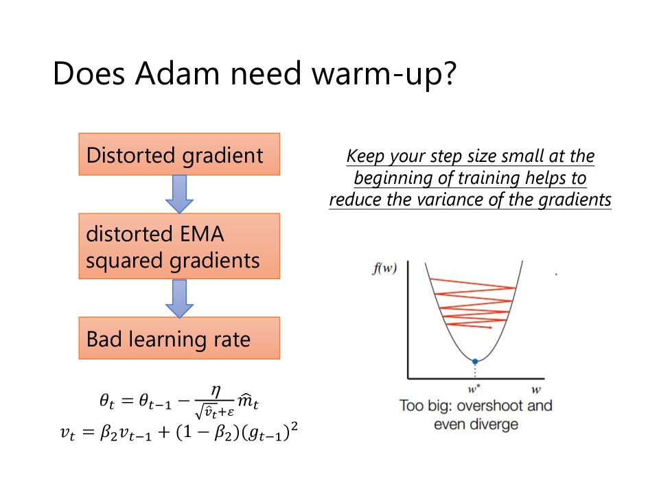
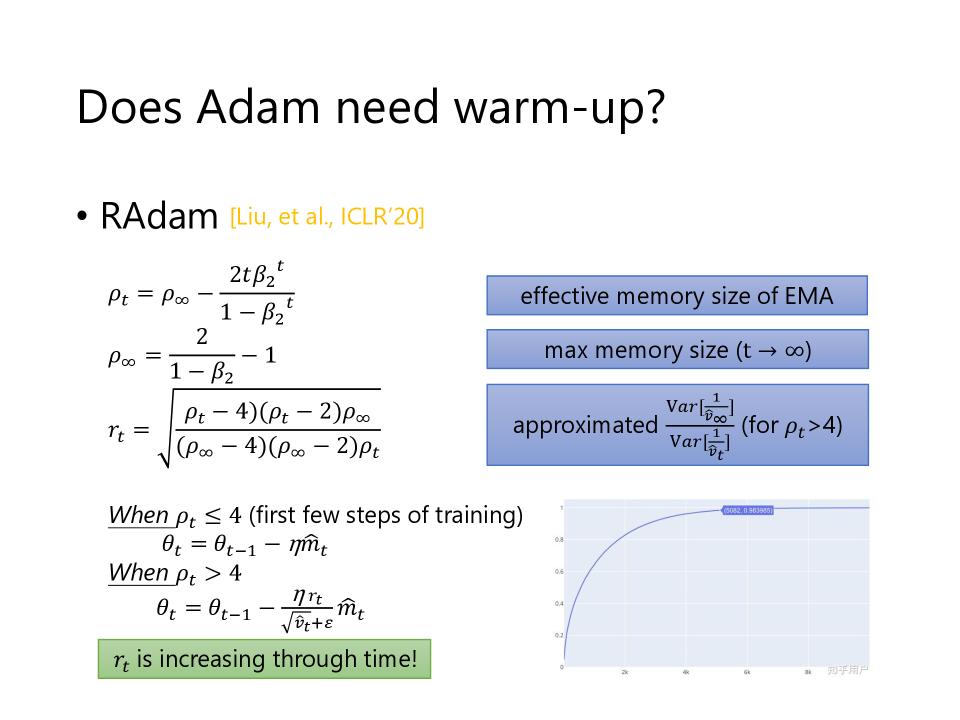
Does Adam need warm-up?
- distorted(扭曲的) gradient -> distorted EMA squared gradients -> Bad learning rate
- keep your step size small at the beginning of training helps to reduce the variance of the gradients
- 新的warm-up的方法是,先变小,再变大
RAdam
RAdam vs SWATS
| RAdam | SWATS | |
|---|---|---|
| Inspiration 灵感 | Distortion of gradient at the beginning of training results in inaccurate adaptive learning rate 训练开始时梯度失真导致自适应学习率不准确 | non-convergence and generalization gap of Adam, slow training of SGDM Adam 的不收敛和泛化差距,SGDM 训练缓慢 |
| How | Apply warm-up learning rate to reduce the influence of inaccurate adaptive learning rate 应用预热学习率减少自适应学习率不准确的影响 | Combine their advantages by applying Adam first, then SGDM 通过先应用 Adam,然后应用 SGDM 来结合它们的优势 |
| Switch | SGDM to RAdam | Adam to SGDM |
| Why switch | The approximation of the variance of $\hat{v}_t$ is invalid at the beginning of training 方差的近似值$\hat{v}_t$在训练开始时无效 | To purse better convergence 追求更好的收敛 |
| Switch point | When the approximation becomes valid 当近似值成立时 | Some human-defined criteria 一些人为定义的标准 |
K step forward, 1 step back
- Lookahead: universal wrapper for all optimizers
- 这个算法有两组weight:
- 这里$\theta$是用于explore(探索)的,叫做Fast weights
- $\phi$是真正需要的weight,叫做Slow weights
- 循环分外循环和内循环。
- 内循环会走k步,内循环的Optim可以使用任意的optimizer
- 每走完一遍内循环,根据当前位置,到内循环开始前的位置,根据$\alpha$计算出下次循环开始的位置
- 接下来,使用新计算出来的$\phi$进行新一轮的内循环
- 这个方法和Memo里面的演算法Reptile很像
\begin{align} & \text{For }t = 1, 2, \dots \text{(outer loop)} \cr & \theta_{t,0} = \phi_{t-1} \cr & \text{For } i = 1, 2, \dots, k \text{(inner loop)} \cr & \theta_{t,i} = \theta_{t, i-1} + \text{Optim(Loss, data, }\theta_{t, i-1}\text{)} \cr & \phi_t = \phi_{t-1} + \alpha(\theta_{t,k} - \phi_{t-1}) \end{align}
- 1 step back: avoid too dangerous exploration, 避免走入一个峡谷的minima
- Look for a more flatten minimum, 寻找更多的平坦的minima
- More stable
- Better generalization

More than momentum
Can we look into the future?
- Nesterov accelerated gradient (NAG)
- SGDM
- $ \theta_t = \theta_{t-1} - m_t $
- $ m_t = \lambda m_{t-1} + \eta \nabla L (\theta_{t-1}) $
- Look into the future
- $ \theta_t = \theta_{t-1} - m_t $
- $ m_t = \lambda m_{t-1} + \eta \nabla L (\theta_{t-1} - \lambda m_{t-1}) $
\begin{align} \text{Let } {\theta_t}^\prime &= \theta_t - \lambda m_t \cr &= \theta_{t-1} - m_t - \lambda m_t \cr &= \theta_{t-1} - \lambda m_t - \lambda m_{t-1} - \eta \nabla L(\theta_{t-1} - \lambda m_{t-1}) \cr &= {\theta_{t-1}}^\prime - \lambda m_t - \eta \nabla L({\theta_{t-1}}^\prime) \cr m_t &= \lambda m_{t-1} + \eta \nabla L({\theta_{t-1}}^\prime) \end{align}
Adam in the future
- Nadam
- $ \theta_t = \theta_{t-1} - \frac{\eta}{\sqrt{\hat{v}}+\varepsilon} \hat{m}_t $
- $ \hat m_t = \frac{\beta_1 m_t}{1-{\beta_1}^{t+1}} + \frac{(1-\beta_1) g_{t-1}}{1-{\beta_1}^t} $
- SGDM
- $ \hat m_t = \frac{1}{1-{\beta_1}^t}(\beta_1 m_{t-1} + (1-\beta_1)g_{t-1}) $
- $ = \frac{\beta_1m_{t-1}}{1-{\beta_1}^t} + \frac{(1-\beta_1)g_{t-1}}{1-{\beta_1}^t} $
Do you really know your optimizer?
- A story of L2 regularization
- AdamW & SGDW with momentum
- SGDWM
- AdamW
Something helps optimization
增加随机性的方法
- Shuffling
- Dropout: 增加随机性的方法
- Gradient noise: 在计算Gradient后,加上一个高斯的noise
和Learning Rate调整相关的方法
- Warm-up
- Curriculum learning: 比如使用没有噪音的声音去训练它,等到它足够强的时候,再融入有噪音的训练样本。
- Train your model with easy data(e.g. clean voice) first, then difficult data.
- Perhaps helps to improve generalization.
- Fine-tuning
Normalization
- Batch Normalization
- Instance Normalization
- Group Normalization
- Layer Normalization
- Positional Normalization
Regularization
Optimize method
- Team SGD
- SGD
- SGDM
- Learning rate scheduling
- NAG
- SGDWM
- Team Adam
- Adagrad
- RMSProp
- Adam
- AMSGrad
- AdaBound
- Learning rate scheduling
- Radam
- Nadam
- AdamW
- SWATS
- Lookahead
| SGDM | Adam |
|---|---|
| Slow | Fast |
| Better convergence | Possibly non-convergence |
| Stable | Unstable |
| Smaller generalization gap | Larger generalization gap |
- SGDM
- Computer vision
- image classification
- segmentation
- object detection
- Adam
- NLP
- QA
- machine translation
- summary
- Speech synthesis
- GAN
- Reinforcement learning
- NLP