Fat vs Deep Network
全量空间与样本空间
- 全量空间(理想状态): If we can collect all datasets in the universe $ D_{all} $, we can find the best threshold $h^{all}$
- $ h^{all} = \text{arg}\min\limits_h L (h, D_{all}) $
- 样本空间(现实发生): We only collect some examples $D_{train}$ from $D_{all}$
- $ D_{train} = {(x^1, \hat{y}^1), (x^2, \hat{y}^2), \dots, (x^N, \hat{y}^N)} $
- $ (x^n, \hat{y}^n) \sim D_{all} $, 采样满足independently and identically distributed (i.i.d.)特性
- 通过$ D_{train} $找到最小Loss的那个h,叫$ h^{train} $: $ h^{train} = \text{arg}\min\limits_h L(h, D_{train}) $
- In most applications, you cannot obtain $ D_{all}$. (Testing data $D_{test}$ as the proxy of $D_{all}$)
We hope $ L({\color{blue}h^{train}}, {\color{red}D_{all}}) $ and $ L({\color{red}h^{all}}, {\color{red}D_{all}}) $ are close.
We want $ L({\color{blue}h^{train}}, {\color{red}D_{all}}) - L({\color{red}h^{all}}, {\color{red}D_{all}}) \leq \delta $
How to make $ P(D_{train} \text{ is bad}) smaller $
- $ P(D_{train} \text{ is bad}) = |H| \cdot 2exp(-2N\varepsilon^2) $
- Larger N and smaller $ |H| $, 样本空间数量尽可能大,全量空间数量尽可能小
If we want $ P(D_{train} \text{ is bad}) \leq \delta $
- How many training examples do we need?
- $ |H|\cdot 2exp(-2N\varepsilon^2) \leq \delta \Rightarrow N \geq \frac{log(2|H|/\delta)}{2\varepsilon^2} $
# 假设 H = 10000, delta = 0.1, epsilon = 0.1
import math
math.log(2*10000/0.1, math.e)/(2*0.1**2)
# output is: 610.3036322765086
Tradeoff(权衡) of Model Complexity
- Larger N and smaller $|H| \Rightarrow L(h^{train}, D_{all}) - L(h^{all}, D_{all}) \leq \delta $
- Smaller $ |H| \Rightarrow \text{Larger }L(h^{all}, D_{all})$
Why Hidden Layer?
- Piecewise Linear
- We can have good approximation with sufficient pieces.
- piecewise linear = constant + sum of a set of
Hard Sigmoid - or use two
Rectified Linear Unit (ReLU)instead of oneHard Sigmoid
- 一层的Piecewise Linear就可以模拟出任何的函数,那么为何需要多层呢?
- Why we want “Deep” network, not “Fat” network?
Deeper is Better?
- 下面列出了层数与正确率的列表,左边Thin + Tall;右边Fat + Short
- 表格中5X2k的参数量与3772相当,所以放在一起做个比较
- 从表格中可以的出结论,在参数量相当的情况下,瘦高型要好于矮胖型
| Layer X Size | Word Error Rate(%) | Layer X Size | Word Error Rate(%) |
|---|---|---|---|
| 1 X 2k | 24.2 | ||
| 2 X 2k | 20.4 | ||
| 3 X 2k | 18.4 | ||
| 4 X 2k | 17.8 | ||
| 5 X 2k | 17.2 | 1 X 3772 | 22.5 |
| 7 X 2k | 17.1 | 1 X 4634 | 22.6 |
| 1 X 16K | 22.1 |
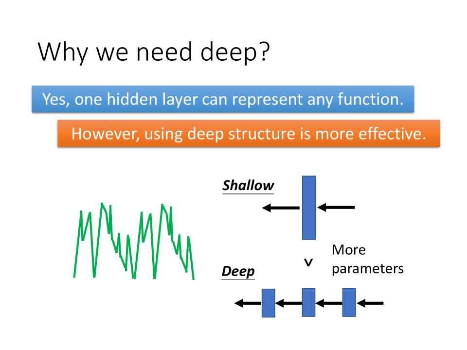
Why we need deep ?
- yes, one hidden layer can represent any function.
- However, using deep structure is more effective.
- 产生相同的function,Shallow的参数数量要多于Deep的。
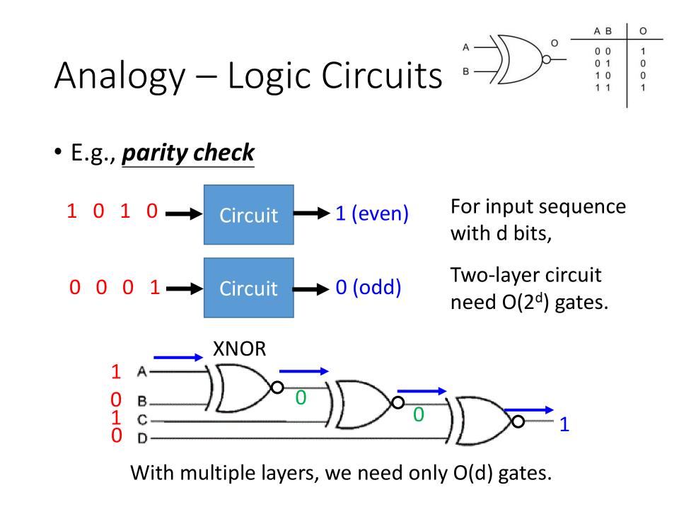
Analogy - Logic Circuits
- parity check (奇偶校验)
- For input sequence with
dbits, 假设此处d=4。 - Two-layer circuit need O($2^d$) gates: O = 16
- 或者,3个XNOR的gates也可以达到相同的效果
- With multiple layers, we need only O(d) gates:O = 4
- For input sequence with
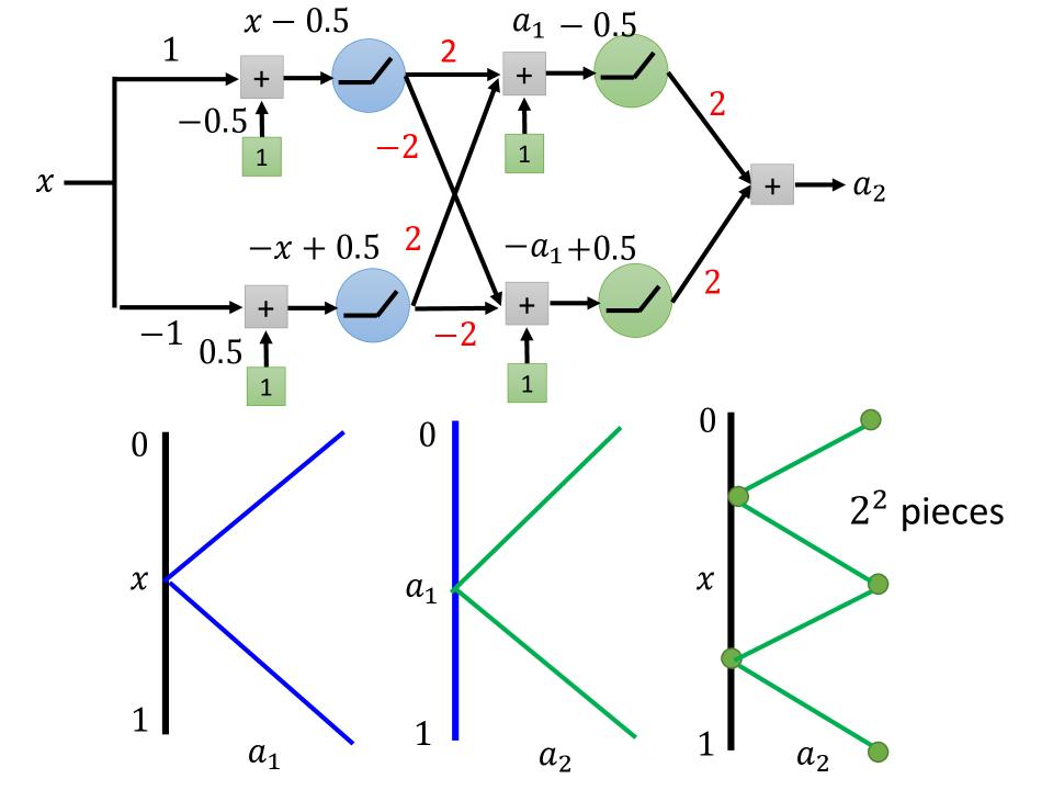
Use Neuron Network
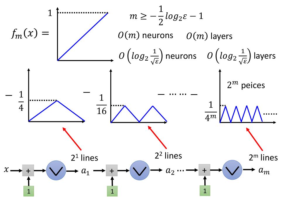
$2^2$ pieces
- 如图,假设图中所用activation function为ReLU
- 图中所画图形需要旋转90度,将x作为横轴来看
- x与$a_1$的关系是,当x从0-1时,$a_1$先下降(从1-0)后上升(从0-1)
- $a_1$与$a_2$的关系是,当$a_1$从0-1时,$a_2$先下降(从1-0)后上升(从0-1)
- x与$a_2$的关系, 会得到4个线段
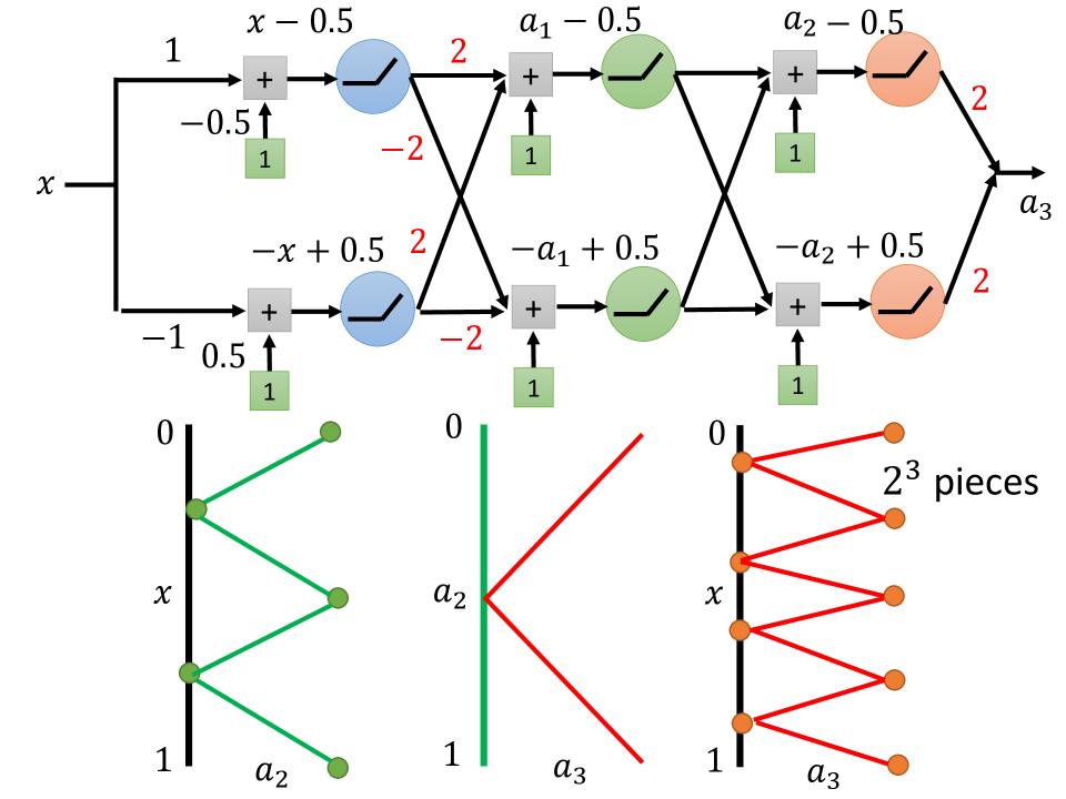
$2^3$ pieces
- 接上步, x与$a_2$的关系, 会得到4个线段
- $a_2$与$a_3$的关系是,当$a_2$从0-1时,$a_3$先下降(从1-0)后上升(从0-1)
- x与$a_3$的关系, 会得到8个线段
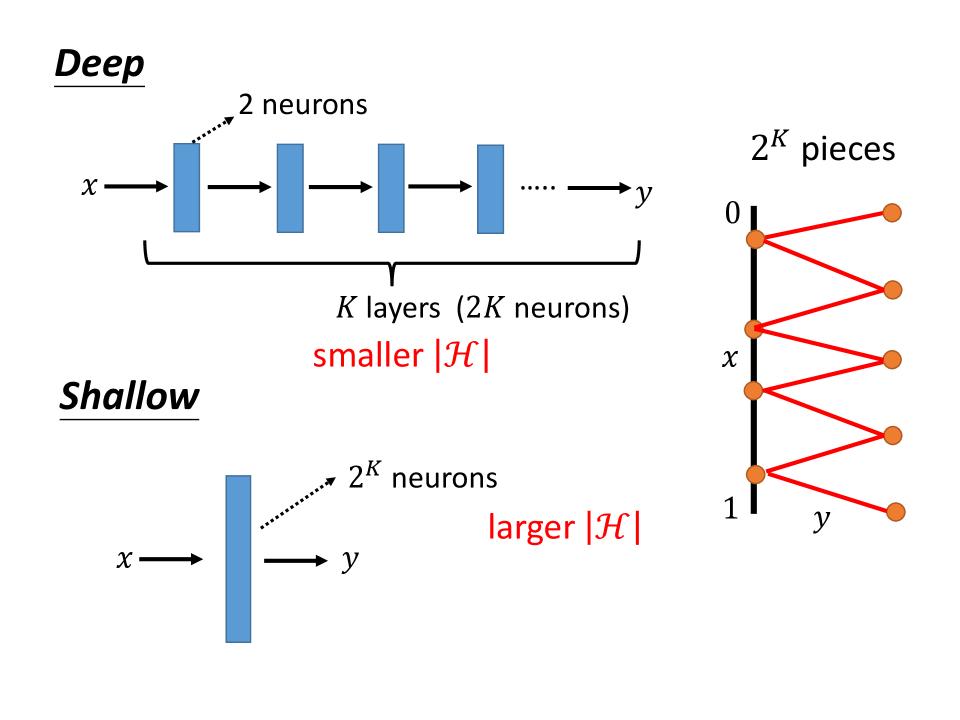
$2^k$ pieces
- 假设在x从0-1的变化过程中,需要让一个nn的output y有$2^k$的线段
- 使用deep的方式,那么只需要k层,每层2个neurons,总共2K个neurons就可以满足需要
- 使用shallow的方式,那么需要$2^k$个neurons才能满足需要
- 所以要产生同样的function
- Deep: 参数量比较小,smaller $|H|$; 模型比较简单
- Shallow: 参数量比较大,larger $|H|$;模型比较复杂
- 在样本数相同的情况下,复杂的模型比较容易overfitting
Think more
- Deep networks outperforms shallow ones when the required functions are
complex and regular.- Image, speech, etc. have this characteristics.
- 当所需功能“复杂且有规律”时,深度网络优于浅层网络。
- Deep is exponentially better than shallow even when $ y = x^2 $
I used a validation set, but my model still overfitted
- 什么时候理想和现实会有差距
- 抽到一个不好的training(validation)data的时候,会有较大的差距(overfitting)
- 模型比较复杂
- 待选择的模型太多了,也可能overfitting
Can shallow network fit any function
- network structure: 网络架构,决定了网络怎么连接
- 同样的structure,填入不同的参数(填入不同的weight和bias),得到不同的function,即一个function space(/set)
deep vs shallow
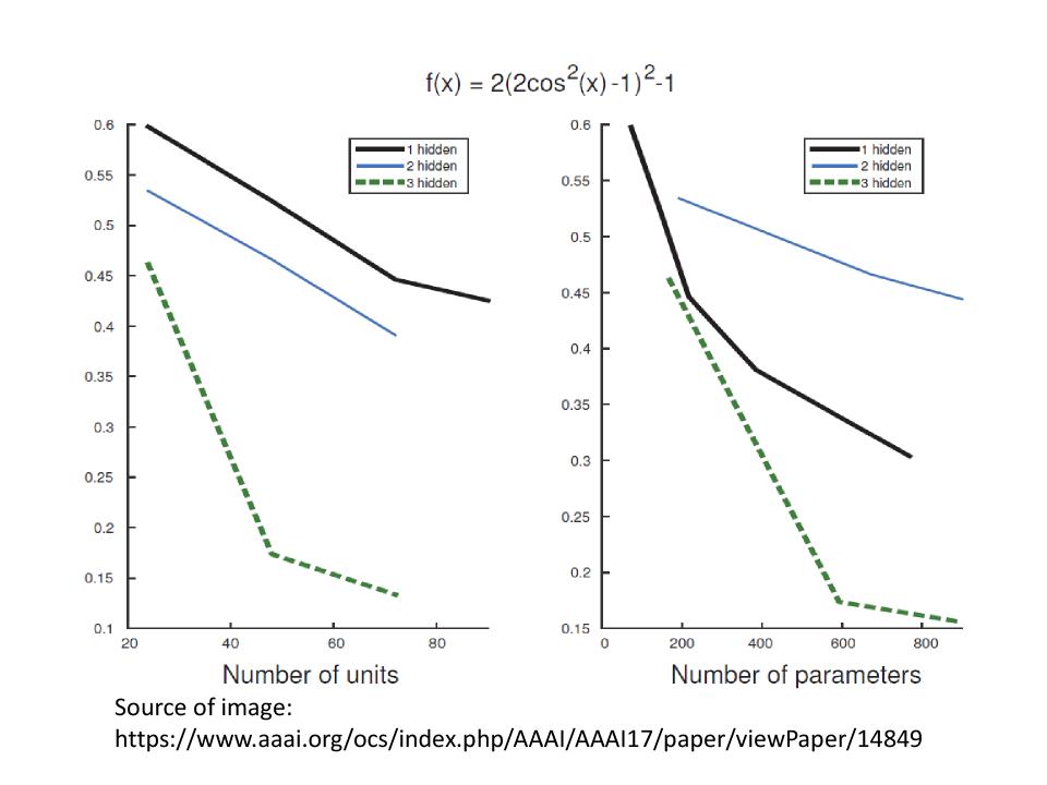
- 假设一个function: $ f(x) = 2(2cos^2(x)-1)^2-1 $, 如下图
- 图中不同颜色的线段代表不同的hidden层数
- 横坐标表示units(/parameters)的数量,纵坐标表示对应的loss
- 从图中可以看出在相同参数量的情况下,deep越深,loss越小(fit越好)
- 相应的当观察相同loss的情况下,deep越深参数量越小
- 注:unit的数目就是neuron的数目,用neuron的数目表示一个network的架构,neuron的数目和parameter的数目是正相关的
- 假设一个目标function: $ y = x^2 $
- 假设一个small的shallow的function,可能并不能很好的fit到这个function,只有当这个shallow的参数足够large的时候,才能找到有效的function
- 而deep去fit同样的function,需要的参数是少的
Universality
- Given a shallow network structure with one hidden layer with ReLU activation and linear output
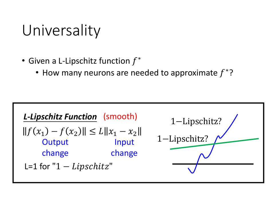
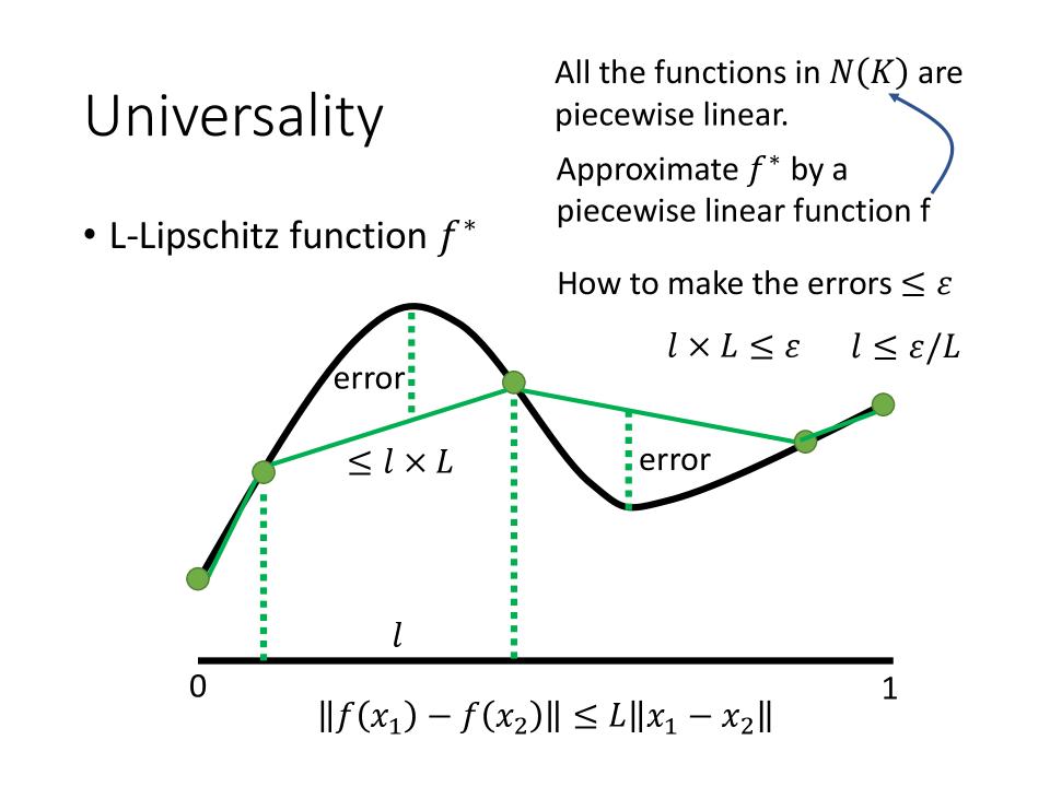
- Given a L-Lipschitz function $f^*$
- How many neurons are needed to approximate $f^*$?
- L-Lipschitz Function (smooth)
- $ || f(x_1) - f(x_2) || \le L || x_1 - x_2 || $
- 左边是Output change, 右边是Input change
- L = 1 for “1-Lipschitz” function; 当L取1时,式子表示为:$ || f(x_1) - f(x_2) || \le || x_1 - x_2 || $, 即输出的变化不能大于输入的变化
- L = 2 for “2 - Lipschitz” function
- 下图,蓝色变化比较快的就不是1-Lipschitz function,而绿色的是1-Lipschitz function
- How many neurons are needed to approximate $f^*$?
- Given a L-Lipschitz function $f^*$
- How many neurons are needed to approximate $f^*$?
- $ f \in N(K) \Rightarrow {\color{green}\text{The function space defined by the network with K neurons.}} $
- Given a small number $\epsilon > 0$, what is the number of K such that
- Exist $ f \in N(K), \max\limits_{0 \le x \le 1}|f(x) - f^*(x)| \le \epsilon $
- The difference between $f(x)$ and $f^*(x)$ is smaller than $\epsilon$.
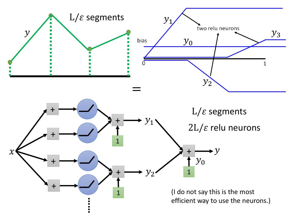
- All the functions in N(K) are piecewise linear.
- Approximate $f^*$ by a piecewise linear function f
- How to make the $ errors \le \epsilon $
- 如下图:$ l = ||x_1 - x_2 || $, $ error = || f(x_1) - f(x_2) || $
- 由L-Lipschitz function得到: $ || f(x_1) - f(x_2) || \le L || x_1 - x_2 || \le \epsilon \Rightarrow error \le l \times L \le \epsilon \Rightarrow error \le \epsilon $
- 则: $ l \times L \le \epsilon \Rightarrow l \le \epsilon / L $
- How many neurons are needed to approximate $f^*$?
- 结合上面推到,下面图可以得到如下结论:
- 当x的取值是[0, 1]: $ segments = L/\epsilon $
- 每一段L-Lipschitz function是由2个ReLU neurons组成,即: $ \text{relu neurons} = 2L/\epsilon $
Potential of Deep
Why we need deep?
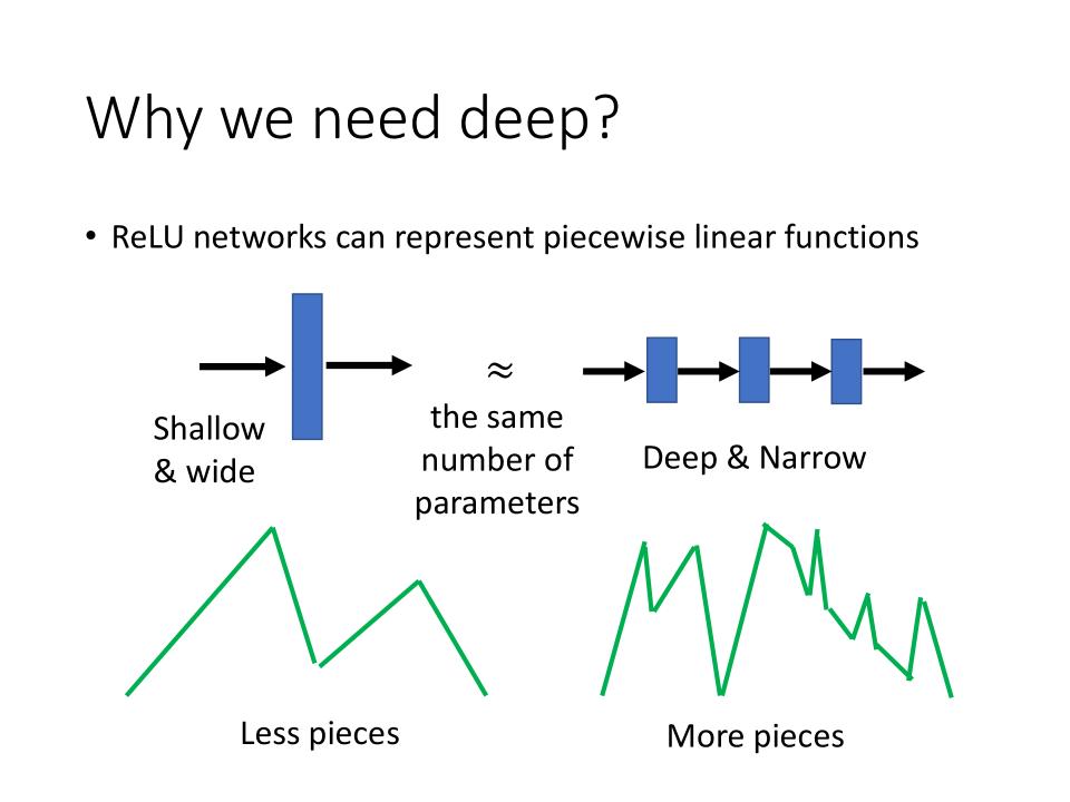
- ReLU networks can represent piecewise linear functions
- same number of parameters with Shallow & Wide will have Less pieces.
- same number of parameters with Deep & Narrow will have More pieces.
Upper Bound of Linear Pieces
- Each “activation pattern” defines a linear function
- ReLU的network,每一个neuron有两个operation的region;一个region的output是0,另一个region的input等于output。
- activation pattern: 某一种neuron的mode的组合
- 假设有n个neuron,且每个neuron为并联(shallow & wide),则最大有n+1个piecewise
- 假设有n个neuron,且每个neuron为串联(deep & narrow),则最大有$2^N$个piecewise
下面代码说明shallow & wide的网络的piece数(upper_bound_test.py):
import numpy as np
import matplotlib.pyplot as plt


def relu(x):
    return (np.maximum(0, x))


def upper_bound_test(x):
    y1 = relu(x * 1 + 1)
    y2 = relu(x * 1 - 1)
    y3 = relu(x * 1 + 0)

    return (y1 + y2 + y3) * 1 + 0


if __name__ == '__main__':
    x = np.linspace(start=-2, stop=2, num=41)
    y = upper_bound_test(x)
    plt.plot(x, y)
    plt.show()
下面代码说明deep & narrow的网络的piece数(abs_activation_test.py):
- 每个layer有2个ReLU组成一个abs activation function, 每个layer有2个region
- 当有3层layer时,有$2^3$的region(piecewise linear)
- deep成立的先决条件是,同样的pattern,反复的出现
import numpy as np
import matplotlib.pyplot as plt


def relu(x):
    return (np.maximum(0, x))


def abs_activation(x):
    y1 = relu(x * 1 - 0.5)
    y2 = relu(x * -1 + 0.5)

    return (y1 + y2) * 2 + 0


if __name__ == '__main__':
    layer_number = 3
    x = np.linspace(start=0, stop=1, num=1001)
    y = x
    for _ in range(layer_number):
        y = abs_activation(y)
    plt.plot(x, y)
    plt.show()
Lower Bound of Linear Pieces
- If K is width, H is depth. We can have at least $K^H$ pieces.
使用MNIST进行实验,得到如下结论
- 当宽度固定,不断的增加深度,则piece按照指数递增
- 当层数固定,而增加每层的宽度,piece的增加并不明显
- 当输入是一个二维的圆圈,在一个100个layer上的network得到的piece,每一层都会是一个对称的图形
- 越接近输入端的layer就越重要
Using deep structure to fit functions
假设需要fit一个简单的function $ f(x) = x ^ 2$
- $f_m(x)=2^m$, a function with $2^m$ pieces
- $ \max\limits_{0 \le x \le 1} | f(x) - f_m(x) | \le \epsilon $
- the minimum m is: $ m \ge -\frac{1}{2}log_2\epsilon -1 $
$ f(x) = x ^ 2$对应的是下图两个线段相减
Why care about $ y=x^2 $
- $ y=x^2 $ : Square Net
- 有了
Square Net,就有了Multiply Net。$ y = x_1 x_2 = \frac{1}{2}((x_1+x_2)^2 - x_1^2 - x_2^2) $ 。运用三个Square Net,可以得到一个Multiply Net。 - 有了
Square Net和Multiply Net就可以做Polynomial(多项式)。
Deep better than Shallow
- The Power of Depth for Feedforward Neural Networks, COLT, 2016:
- A function expressible by a 3-layer feedforward network cannot be approximated by 2-layer network.
- Unless the width of 2-layer network is VERY large
- Applied on activation functions beyond relu
- The width of 3-layer network is K.
- The width of 2-layer network should be $Ae^{BK^{\sfrac{4}{19}}}$
- A function expressible by a 3-layer feedforward network cannot be approximated by 2-layer network.
- Benefits of depth in neural networks, COLT, 2016.
- A function expressible by a deep feedforward network cannot be approximated by a shallow netowrk.
- Unless the width of the shallow network is VERY large
- Applied on activation functions beyond relu
- A function expressible by a deep feedforward network cannot be approximated by a shallow netowrk.
- Depth-Width Tradeoffs in Approximating Natural Functions with Neural Networks, ICML, 2017
- 一个球形,3-layer, width 100, is better than 2-layer, width 800
- Error bounds for approximations with deep ReLU networks, arXiv, 2016
- Optimal approximation of continuous functions by very deep ReLU nertworks, arXiv 2018
- Why Deep Neural Networks for function Approximation?, ICLR, 2017
- Depth-width Tradeoffs in Approximating Natural Functions with Neural Networks, ICML, 2017
- When and Why Are Deep Networks Better Than Shallow Ones?, AAAI, 2017